
With SharpCap 3.1 now ready for release, here’s a quick rundown of the new features and improvements that have been added.
Mini Histogram
Something I probably should have added long ago – an always on mini histogram in the control panel that’s integrated with an easy-to-use way of stretching the image for display to bring out the fainter details…

This doesn’t have all the power of the main histogram – for instance it only updates a couple of times per second to conserve resources and it doesn’t support the selection area option, so it always shows the histogram of the entire frame, but it makes up for that by always being available.
As well as being able to inspect the image histogram, you can tweak the display stretch function by dragging the three dashed vertical lines that indicate the black point, mid point and white point. These adjustments make it very easy to pull out faint detail on the screen (they don’t affect data being saved to file). You can also use the auto stretch button (the lightning bolt) to have SharpCap automatically stretch the image for you and also reset the stretch back to default using the reset button. To round things off, the intensity of the auto stretch is configurable in the SharpCap settings, so you can pick an auto-stretch intensity that works for you.
Note that the mini histogram does not require a SharpCap Pro license, but the use of the auto stretch button does.
Auto Restore of Camera Settings
SharpCap 3.1 automatically saves camera settings when you close a camera and then restores them the next time you open that camera. This behavious is enabled by default, but if you prefer to return to the old way of working, the auto-restore can be disabled in ‘general’ tab of the SharpCap settings.
If you need to stop the settings from being restored on a particular occasion, but don’t want to turn this feature off completely, then simply hold down <CTRL> while opening the camera to disable settings restore temporarily.
Smart Histogram
Ever wondered whether you are using the right gain or exposure when deep sky imaging? Whether 6x ten minute exposures really do give you more detail than 12x five minute exposures? No more guesswork required with the new SharpCap Pro Smart Histogram feature. In combination with the results of Sensor Analysis (see below), SharpCap can measure the sky background brightness for you and then perform a mathematical simulation of the impact on final stacked image quality of using different gain and exposure combinations. You can also see graphs showing the impact of using longer or shorter exposures (or lower or higher gain) than suggested.
If you try this using a modern, low noise, CMOS sensor you might be pleasantly surprised to find out that the optimal exposure length isn’t nearly as long as you imagine and that maybe the complexities of guiding will become a thing of the past (The use of long – 5 to 10 minute or even longer – exposures in traditional deep sky imaging is not required to see faint targets, it’s actually required to deal with the high typical read noise of CCD sensors. Since the optimal exposure length is proportional to the square of the read noise and CMOS read noises can be 1-3 electrons instead of 8-10, exposures can often be much shorter with no loss of quality).
The basic form of Smart Histogram takes the form of a pair of coloured bars along the top of the histogram area :

The top bar with the red, amber and green sections shows the impact of your camera’s read noise on the total image noise at that brightness level. For areas of the image in the red highlighted region of the histogram, the camera read noise dominates the total noise (>50% of total noise). In the amber region, the read noise contributes significantly to the total noise (10% to 50%). In the green region, the contribution from read noise is small (<10%). The size of the red and orange zones will vary as you vary the gain and offset controls of your camera. Once you have picked values for those controls, you should adjust the exposure so that the histogram peak corresponding to the sky background is just to the right of the orange zone – this will give you optimum image quality without entering the zone where increased exposure time has diminishing (to zero) returns.The lower bar indicates the effect of bit depth on the quality of captured image. In high bit depth modes (12, 14, 16 bit), the bar is green and light green – the light green section shows the range where the increased bit depth is not helping you because the total pixel noise equals or exceeds the distance between ADU levels in 8 bit mode. In the light green region, the use of high bit depth simply means that you are recording the pixel noise in greater detail!
In 8 bit modes, the lower bar is amber and green :
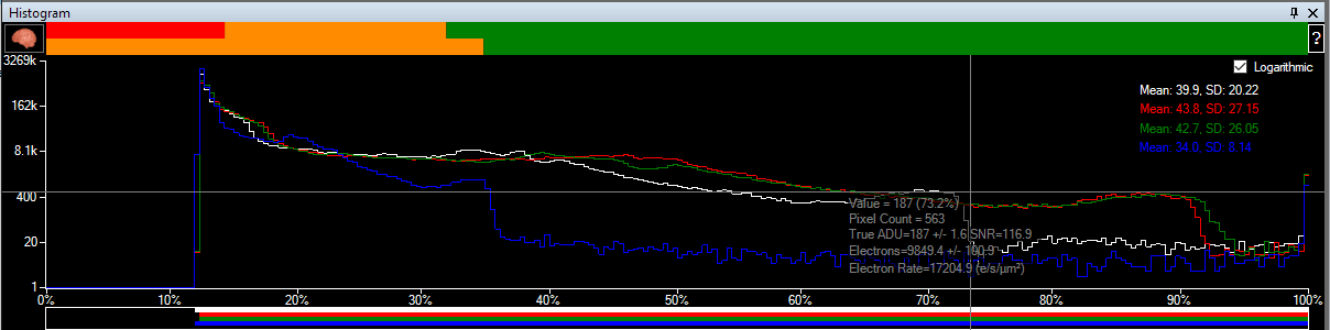
The amber region indicates the part of the histogram where you are throwing away data by using 8 bit mode (ie you would get more image quality by switching to 12/14/16 bits for parts of the image in this histogram region). The amber region will shrink to the left as you increase the camera gain level, and at the high gains used in planetary imaging it may not be visible at all – this shows why there is no need to use high bit depth modes for planetary ‘lucky’ imaging (and also that the Smart Histogram isn’t only useful for deep sky!).
The coloured bars at the top of the histogram are just the ‘quick’ way to use the Smart Histogram features, giving you some basic guidance on exposure times and bit depths. For a more in-depth calculation that gives recommendations on gain, offset, exposure and bit depth, press the ‘Brain’ button next to the coloured bars to bring up the Brain window.
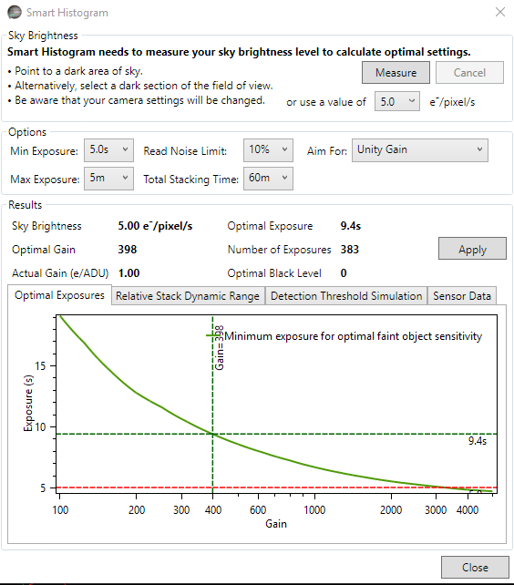
The ‘Brain’ window is quite complicated, but if you follow it from top to bottom it should not be too hard to use.
The goal of the Brain is to help you pick the right camera settings to get the best deep sky images. Note that the Brain is *not* aiming to give you fabulous quality sub-exposure images, it is calculating how to get the best final image when you stack all frames taken in a set period of time (1 hour by default). The calculations will work out for you whether it is better to take 360 x 10 second images or 10 x 360 second images or some other combination.
The first step is to measure (or enter) your sky brightness – this is measured in electrons per pixel per second and is a measure of how much signal is arriving at every pixel on your camera every second from sources that we don’t really want – light pollution and thermal noise being the main culprits. If you press the ‘Measure’ button then SharpCap will set the gain to maximum and take a number of increasing length exposures to measure this value – you should point the telescope at an area of sky without nebulosity or many stars to get a good measurement.
The next step is to set limits and targets for the calculation – you can set a minimum and maximum exposure to consider (typically maximum exposure is determined by mount tracking/guiding quality and minimum by how much data you have to save with very short frames or stacking speed for live stacking). You can also set the time you intend to image for (not critical, changing this will *not* change the suggested values) and the contribution you are prepared to tolerate from the sensor read noise in the final image noise level. If you select a ‘Read Noise Limit’ of 10%, that means that the calculations will allow the total noise level in the final stacked image to increase by 10% above the minimum achievable noise level (ie to go from 10 to 11 on some scale).
The last choice in this section determines how the gain is chosen – the two options are ‘Unity Gain’ which aims for 1 electron per ADU (or as close as possible) and ‘Max Dynamic Range’. ‘Max Dynamic Range’ finds the gain where the final stacked image will have the maximum ratio between the brightest thing that is not quite saturated and the noise level. Max Dynamic Range will often (but not always) choose the minimum gain value.
Once the sky background is measured and the limits and targets are set you can examine the results. In the image above, you can see that with a 5e/pixel/s sky brightness (quite bad light pollution), the calculation is recommending a gain value of 398, an exposure of 9.4s and a black level of zero (because the sky brightness will be enough to pull the histogram clear of the left hand side). The graphs below show useful detail on the calculations that help you understand the result and if necessary tweak the values.
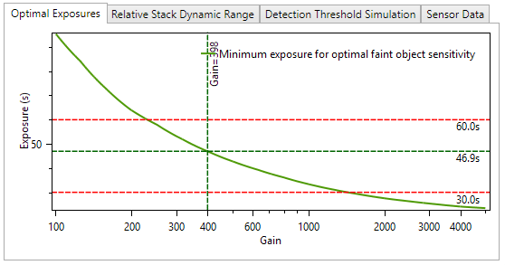
The optimal exposure chart shows you the exposure time you need to use to hit your ‘Read Noise Limit’ criteria for different gains – it also shows your minimum and maximum exposure limits as horizontal red lines if they fall within the range of the graph. From this graph we can see that in this case the recommended exposure is 46.9s at 398 gain, but an exposure of 60s could be used at 230 gain or 30s at about 1400 gain to get very similar results. You aim for at least the exposure time shown on this graph, although selecting a longer exposure won’t improve things much as we will see in the detection threshold simulation chart.

The relative stack dynamic range chart shows how the dynamic range of the final stacked image will be affected by changing the gain (assuming you follow the suggested exposure time for each gain value). This chart shows information for different bit depths if the required sensor analysis data is available. In this case the stack dynamic range for the 8 bit line drops to zero at gains below about 450. This happens when there are no valid solutions for the exposure time that fit all the limits you have chosen – for instance in this case a read noise limit of 10% would require exposures longer thant the maximum exposure value of 5 minutes when in 8 bit mode with a gain < 450. In this case (in common with many cameras), you can get a slight increase in the dynamic range of the final stacked image by moving to lower gain values.
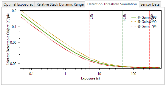
The third chart shows how the faintest visible object in the final stacked image varies with different exposure times. This chart makes it very clear how little extra you will achieve (other than pain in terms of guiding, tracking, hot pixels, satellite trails, aeroplane trails, etc) by exceeding the recommended exposure times. In this case at the recommended values, the expected faintest detectable object would be 0.0176 e/pixel/s. Increasing the exposure from ~47s to 300s drops that to 0.0168 e/pixel/s, an improvement of about 5%. You can also see that by this point the curves are basically flat – further increases in exposure bring practically no improvement to the final stacked image…
The Detection Threshold Simulation assumes that the faintest object you will be able to see in the final stacked image is equal in brightness to the noise level in that image. In fact, for objects that cover a large number of pixels, you might do a bit better than that as it is easier to see a large faint object than a small one, but this does not change the shape of the curve, in particular the fact that beyond the recommended exposure level there is practically no improvement in final image quality with further exposure increases.
In summary, when you use the Brain window, SharpCap simulates in a fraction of a second all the possible combinations of gain and exposure that you might use to image and calculates what the effect of each set of parameters would be on the final stacked image. This is possible because the results of the Sensor Analysis allow SharpCap to calculate the behaviour of the sensor for any combination of gain and exposure.
Smart Histogram requires a SharpCap Pro license and you must perform sensor analysis on each model of camera you intend to use. For best results perform sensor analysis in both 8 bit and high bit depth (12/14/16) modes.
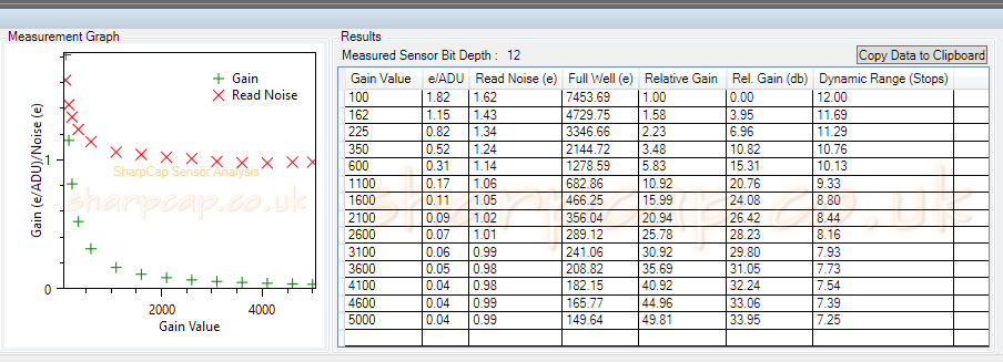
Sensor Analysis
Ever seen those graphs provided by camera manufacturers of Sensor gain and read noise? Wondered how they were created? Well, they used to be a lot of manual adjustments and tedious measurements and calculations, but now SharpCap can perform those measurements automatically for you to generate a custom sensor analysis of your very own camera.
Why would you want to do that? Because the sensor data that is produced feeds into the SharpCap Smart Histogram functionality, which provides accurate guidance on the best gain/exposure to use for deep sky imaging based on the characteristics of your imaging sensor. With those numbers, SharpCap can perform a mathematical simulation of the amount of image noise that would occur in a whole range of different gain and exposure values and guide you to the ones that will give the best result.
Run a sensor analysis (Tools Menu) on your camera in RAW8 and RAW12/16 mode (or MONO8 and MONO12/16 for mono sensors) and SharpCap will save the results and use them to provide Smart Histogram guidance in future imaging sessions.
Note that SharpCap requires fine control over the camera exposure to perform Sensor Analysis – this means that it’s not possible on Webcams or Frame Grabbers. Also, if you have a colour camera it must be in a RAW mode to perform sensor analysis as the debayer process used to convert RAW images into RGB or MONO images causes sensor analysis to give incorrect results.
Sensor analysis is a free feature and does not require a SharpCap Pro license.
Feature Tracking
This lets SharpCap use your connected ASCOM mount (or ST4 connected camera) to guide the telescope and track on screen image features. Currently it is designed to work with high speed (Solar/Lunar/Planetary) imaging. SharpCap analyzes several frames per second and tracks movement of features between those frames – when the movement exceeds a threshold it will begin to make adjustments to bring the image back to it’s original position. An initial calibration step must be performed so that SharpCap can learn which way and how fast the image moves for the various mount movement directions.
Feature Tracking is currently experimental – please feel free to test and report any issues. More feedback on the performance with different mounts and focal lengths is welcome.
Feature Tracking is a SharpCap Pro feature and can be started from the Tools menu.
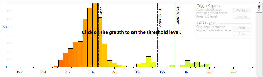
Seeing Monitoring and Auto Capture
This is a new application of the image quality measurement techniques that SharpCap has provided to assist focusing for some time. Instead of helping you find the point of best focus, you can now use the image sharpness measurements to help you capture the moments of clearest seeing without having to sit with your eyes glued to the computer screen at all times.
Launched from the Tools Menu, the seeing monitor shows a chart of the recent range of image quality with the most recent values highlighted. This gives a much more objective measurement of when the seeing is good.
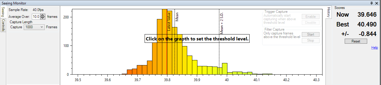
Every new frame is analysed for sharpness (contrast) and the results are added to the graph that will build up below the image. You should select the area you are most interested in using the selection area tool (for instance sunspots, craters). Using the standard colour scheme, sharp frames build the graph in green on the right hand side, poor frames build the left hand side in red. If the seeing is relatively constant then you will see a graph like the one above with a single peak. If the seeing improves or worsens then a new peak will begin to build (to the right for improved seeing, to the left for worse seeing), like the image below. Note that other factors can also change the score and cause a new peak – for instance brightening or dimming caused by passing thin clouds.
SharpCap Pro users can additionally enable two automatic modes:
* Seeing triggered capture – this starts a capture when the seeing value exceeds a user picked threshold
* Seeing filtered capture – this will start a capture but only save the frames that exceed a user picked quality threshold
To enable these, you need to click on the graph to set a threshold level – this is the level which causes either capture to be triggered (when the image quality exceeds the threshold) or causes frames to be saved to file (when using the filtered capture).
Starlight Xpress Camera Supprt
SharpCap 3.1 now supports StarlightXpress cameras natively – no need to use the ASCOM driver any more. This provides better control over the camera and greater reliability. Please report any issues that you have with StarlightXpress cameras on the SharpCap forums.
Other Camera Updates
- Updated SDK for Altair, Basler, Celestron/Point Grey, QHY and ZWO cameras to support new models and fix bugs
- Support for QHY CCD cameras (QHY10 etc) that do not support video mode
- Simplified support for Basler cameras – now a single camera choice provides the full range of available exposures, rather than having to choose between a Normal and LX mode option for the camera
- Improvements to allow more Celestron/Point Grey cameras to work correctly.
- Increased capture limits to a maximum of 100000 for sequence length and 999999 frames in a single capture (probably not useful both at once!)
Blind Plate Solving
SharpCap 3.0 contained integration to ‘Astrometry.Net’ based local plate solvers, but it required you to have a connected ASCOM mount as it used the mount pointing as an initial estimate of location to allow the plate solve to complete quickly. SharpCap 3.1 also contains blind plate solving (on the tools menu) which does not require a connected mount, it will just run your local copy of AstroTortilla/ASPS/AnSvr on the next frame and show the results in the notification bar.
Filename Templates
Lots of users have asked for little tweaks to be made to the way that capture files are named. Adding more checkboxes and dropdowns to the already complicated file naming tab of the settings wasn’t really an option, so instead I’ve added the ability to completely customize the file naming using filename templates. You’ll find these at the bottom of the filename settings tab and you’ll notice that the templates update automatically if they are disabled and you adjust other settings on the page, which will give you a good idea of what is possible for now.
One thing you may notice is that there is the option to include the current filter name in the filename using the {Filter} tag. If you are not using an ASCOM filter wheel then you can still use this feature by selecting ‘Manual Filter Wheel’ in the hardware settings – this will give you a filter wheel control in the camera controls panel which will not do anything except give a filter name to the file name template.

You can see that each filename template can be made up of tags which are wrapped in ‘{‘ and ‘}’ and text. The tags available include dates, times, camera names, target name, filter name, etc. Please note that using filename templates is an advanced feature and incorrect use can lead to files being overwritten – for instance if you do not include either ‘{Index}’ or ‘{FrameTime}’ in your Sequence template you will find that if you capture 100 frames in PNG format you will only get one file on disk because the file name for each frame will be the same and they will overwrite each other. Keep an eye on the ‘Sample Filenames’ above which show you the results of your templates.
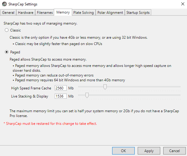
SharpCap Max Memory
This new approach to memory management allows SharpCap to access considerably more system memory if it is available. This reduces the chance of running out of memory when working with high resolutions and allows SharpCap to cache many frames in memory when performing high speed captures (if the Hard Disk can’t keep up).
This feature is only available to users who have 64 bit versions of Windows and at least 4Gb of total system memory.
SharpCap Pro users can allocate up to 50% of their system memory to this feature, so if you have 16Gb of memory you could allocate 8Gb, which would allow SharpCap to cache nearly 6000 1280x1024xRAW8 frames in memory waiting to be written to disk! Non SharpCap Pro users can only allocate 2Gb to this feature, but that still gives a cache of 800+ frames available. The allocated memory needs to be split between high speed imaging frame cache and memory for other tasks such as live stacking on high resolution cameras.
Configure Max Memory settings in the ‘Memory’ tab of the SharpCap settings.
Live Stack Improvements
The Live Stack histogram has a had a significant facelift for this version

As you can see there are now separate traces for the different colour channels and colour balance adjustment sliders available if you are imaging with a colour camera. Note that the histogram always shows the levels of the stack held in memory, so adjustments to the colour sliders and the level stretch do not change this histogram (they do change the way the image looks on screen, how it is saved when using ‘save as seen’ and the mini histogram graph).
The adjustment of the display stretch is also improved and simplified by the removal of the various sliders in verion 3.0 and the addition of 3 simple draggable levels bars to set the black, mid and white points. You can drag these bars using the mouse. If you need very fine control of their position then hold down <SHIFT> while dragging sideways or move the mouse above the graph while dragging sideways – both will cause the bar to move more slowly and give finer control. An auto stretch button (the lightning bolt one) and a reset button complete the improvements to the histogram. It’s much easier now to control how steep the stretch is near the black point, which makes it easier to get good results when applying a strong stretch to faint nebulosity or galaxies.
On the stacking side, addition of a Sigma-clipping stacking option which will help reduce final stack noise and also keep artifacts like satellite, meteor and aircraft trails out of the stacked image (Pro Feature). Please note that changing between the default stacking algorithm and sigma-clipped stacking will reset the current stack. The ‘Stacking’ tab of the Live Stack panel gives some control over the options for the sigma clipped stacking.
There have been considerable improvements to memory usage during Live Stacking which will help with particularly on high resolution cameras. Users of high resolution cameras (10 megapixels or more) should use a 64 bit version of Windows with at least 4Gb of memory (ideally 8Gb+) for live stacking. Users of very high resolution cameras (30 megapixels or more) may need to increase the memory allocated to Live Stacking in the SharpCap memory settings. If PC does not meet this recommended levels then you may find that Live Stacking fails because it runs out of memory – a good workaround to this problem is to use your camera in 2×2 binned mode.
Note that the colour adjustment sliders, auto-stretch button and sigma clipped mode are SharpCap Pro features.
Polar Alignment Improvements
SharpCap 3.1 adds refraction correction to Polar Alignment – this means that SharpCap works out the error introduced by atmospheric refraction of light arriving from stars near the pole and corrects for it. To do this, SharpCap needs to know your correct latitude – this can be specified in the new ‘Polar Alignment’ tab of the settings dialog:
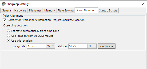
This allows you to turn refraction correction on or off and provide information on your location. If you use an ASCOM mount then SharpCap can retrieve the location from the mount, otherwise you can enter it manually or use the ‘Geolocate’ button if you can connect to the internet. Your location does not need to be exact – to the nearest degree will be fine!
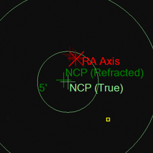
SharpCap 3.1 also introduces some usability improvements to Polar Alignment to help you get great results – these include using a single star for the adjustment guidance (as long as that star stays on screen) and making sure that you don’t see any adjustment instructions until the final adjustment stage has been activated, since adjusting at an earlier stage gives incorrect results.
SharpCap now also tracks the apparent center of rotation position as the rotation angle is increased – this will help spot mechanical issues where the scope mount flexes significantly during rotation leading to poor results. In the images below you can see that the effect of a cable from the guide camera deliberately left unsupported is easily picked up by the red RA axis history crosses forming a line (left image). When the cable is properly tied up the measured RA points form a much tighter cluster (right image).
|
Loose Cable
 |
Secured Cable
 |
The pull of the weight of the dangling cable changes direction as the mount is rotated, moving the guide camera slightly and causing the apparent change in the measured position of the RA axis. To see the history traces for RA position you need to rotate the RA axis slowly (about 15 degrees at a time, then wait for a few frames – the RA axis trace will start to appear after the rotation passes about 30 degrees).
An increased polar alignment star database means that the initial position can be out to about 7 degrees from the pole (previously five degrees).
ASCOM device/camera Improvements
SharpCap 3.1 includes updates to improve compatibility with various ASCOM cameras/focusers/filter wheels and mounts. In particular, you should make sure that you install the ASCOM platform 6.3 (or newer) to get the best results.
A new option is now available in the hardware settings tab that allows you to configure SharpCap *not* to automatically connect to ASCOM hardware (focuser/wheel/mount) when a camera is selected. This is very useful if you do not always use your ASCOM hardware but want to leave it configured for when you do use it. In this mode, ASCOM hardware controls will appear in the control panel, but will not be enabled until the ‘Connected’ check box is ticked.
Other Improvements
- Better control of the zoom level of the preview image. Zoom using the mouse wheel while holding the <CTRL> key down. No flicker of the image while zooming any more
- Scroll the preview image using the mouse wheel if it is bigger than the display area – mouse wheel alone for vertical scrolling, mouse wheel + <SHIFT> for horizontal
- Improved hot pixel handling in Dark Subtraction – SharpCap now analyzes the statistics of the dark frame to select a hot pixel threshold.
- TIFF and JPEG file format output available. Note that JPEG files use lossy compression, so they will be lower quality images. Only use where image file size is important (ie all sky cameras)
- Mean and Standard deviation readouts on the main histogram
- Histogram crosshairs on the main histogram showing level, pixel count and further info if sensor analysis data is available
What has been REMOVED in SharpCap 3.1?
Windows Vista is no longer supported. This is because Windows Vista is too old to recognize the digital signatures that are now used to guarantee the authenticity of each build of SharpCap that you install. I thought it might be possible to make it work if Windows Vista had all possible Windows Updates installed, but I ended up spending 2 days waiting for it to install updates and at the end of that it was still ‘Searching for Updates’. I gave up, sorry.
The ‘old’ way of talking to webcams and frame grabbers that was used in SharpCap 2.9 and earlier (and was available as an option in SharpCap 3.0 – called the ‘DirectShow Pipeline’) is no longer available. Keeping this would have made improvements that needed to be made to the scrolling and zooming of the preview image harder or possibly even impossible.
LX modified webcams – Philips Toucam, SPC900, SPC880, etc – are no longer supported. Support for these devices was tightly linked to the old way of talking to webcams which has also been removed as noted above. If you wish to continue using these devices with SharpCap, please keep version 3.0 installed to support these devices. You can have version 3.0 and 3.1 installed at the same time.